【Matlab 六自由度机器人】运动学逆解（附MATLAB机器人逆解代码）_机器人逆运动学求解matlab-程序员宅基地

技术标签： matlab 算法矩阵线性代数 MATLAB机器人工具箱人工智能

【Matlab 六自由度机器人】求运动学逆解

往期回顾
前言
正文
总结
参考文献

往期回顾

【汇总】

【主线】

【补充说明】

前言

本篇介绍机器人逆运动学及逆解的求解方法，首先介绍如何理解逆向运动学，并利用D-H参数及正向运动学的齐次变换矩阵对机器人运动学逆解进行求解。

在博主读研期间，刚开始对机器人运动学逆解不甚了解，但在经历一次自己完全去钻研、尝试，独立写出属于自己的运动学逆解后，对机器人的结构有更加深刻的理解。因此希望初学机器人的朋友们也能够尝试独立去编写、尝试出自己的逆解代码，我相信，当你看到逆解解出的角度完全符合预期，也能够产生相当的成就感。

下面是运动学逆解的正文内容，主要讲述运动学逆解的方式和公式推算，最后进行代码的实现。

正文

一、运动学逆解

首先我们已经建立起了一个六自由度的机器人，在 D-H 参数及机器人的期望位姿已知的情况下，求解机器人满足该期望位姿的各个关节变量，这种求解过程叫做机器人运动学逆解过程。求解机器人的逆运动学解法分为封闭解法和数值解法两种，其中封闭解法是指具有解析形式的解法，其求解速度比数值解法更快。

本文所研究的六自由度机器人，是具有六个旋转关节的串联型六自由度机器人，即RRR型的机器人。六自由度机器人的逆解封闭解法具体又可分为代数解法和几何解法，代数解法推导解析解的过程复杂，运算量较大，几何解法根据直观的几何关系获得关节变量的解析表达式，计算量较小。

本文主要讲解两种机器人运动学逆解的两种方法：
1. Pieper法
2. 常规法

1. Pieper 法

根据Pieper’s Solution的研究，如果六自由度机器人具有三个连续的轴交在同一点的情况，则手臂具有解析解。即六个关节均为旋转关节且后三个关节轴相交于一点的串联型机器人，其逆解具有封闭解。可以通过如下代数解法求解逆运动学的封闭解，该解法称为“三轴相交的 Pieper 解法”。下面进行各轴转角角度的公式推导。
我们知道，当后3个关节轴相交时，连杆坐标系 ${4\},\{5\},\{6\}$ 的原点位于该交点，该交点在基坐标系 ${0\}$ 中的坐标如下：
$}^{0} \boldsymbol{P}_{4}={ }^{0} \boldsymbol{T}^{1}{ }_{2} \boldsymbol{T}_{3}^{2} \boldsymbol{T}^{3} \boldsymbol{P}_{4}=\left[\begin{array}{llll} x & y & z & 1 \end{array}\right]^{\mathrm{T}}$
对于齐次变换矩阵的变换通式的理解请参阅【Matlab 六自由度机器人】运动学正解（附MATLAB机器人正解完整代码）
由改进D-H参数的连杆齐次变换矩阵式，应用齐次变换矩阵的变换通式

$^{i-1}T_i =\left[ \begin{matrix} cosθ_i&-sinθ_i&0&a_{i-1} \\ sinθ_icosα_{i-1}&cosθ_icosα_{i-1}&-sinα_{i-1}&-sinα_{i-1}d_{i} \\ sinθ_isinα_{i-1}&cosθ_isinα_{i-1}&cosα_{i-1}&cosα_{i-1}d_{i} \\ 0&0&0&1 \end{matrix} \right]$
可知当 $i = 4$ 时，
$}^{0} \boldsymbol{P}_{4}={ }_{1}^{0} \boldsymbol{T}{ }_{2}^{1} \boldsymbol{T}\left({ }_{3}^{2} \boldsymbol{T}^{3} \boldsymbol{P}_{4}\right)={ }_{1}^{0} \boldsymbol{T}{ }_{2}^{1} \boldsymbol{T}\left({ }_{3}^{2} \boldsymbol{T}\left[\begin{array}{c} a_{3} \\ -d_{4} s \alpha_{3} \\ d_{4} c \alpha_{3} \\ 1 \end{array}\right]\right)={ }_{1}^{0} \boldsymbol{T}{ }_{2}^{1} \boldsymbol{T}\left[\begin{array}{c} f_{1}\left(\theta_{3}\right) \\ f_{2}\left(\theta_{3}\right) \\ f_{3}\left(\theta_{3}\right) \\ 1 \end{array}\right]$
应用齐次变换矩阵对于 $}_{3}^{2} \boldsymbol{T}$ 可以得到 $f_{i}$ 的表达式:
$\begin{aligned} &f_{1}=a_{3} c_{3}+d_{4} s \alpha_{3} s_{3}+a_{2} \\ &f_{2}=a_{3} c \alpha_{2} s_{3}-d_{4} s \alpha_{3} c \alpha_{2} c_{3}-d_{4} s \alpha_{2} c \alpha_{3}-d_{3} s \alpha_{2} \\ &f_{3}=a_{3} s \alpha_{2} s_{3}-d_{4} s \alpha_{3} s \alpha_{2} c_{3}+d_{4} c \alpha_{2} c \alpha_{3}+d_{3} c \alpha_{2} \end{aligned}$
对 $}_{1}^{0} \boldsymbol{T}$ 和 $}_{2}^{1} \boldsymbol{T}$ 应用齐次变换矩阵得到
$}^{0} \boldsymbol{P}_{4}=\left[\begin{array}{llll} c_{1} g_{1}-s_{1} g_{2} & s_{1} g_{1}+c_{1} g_{2} & g_{3} & 1 \end{array}\right]^{\mathrm{T}}$
$g_{1} 、 g_{2} 、 g_{3}$ 计算过程如下:
$\begin{aligned} &g_{1}=c_{2} f_{1}-s_{2} f_{2}+a_{1} \\ &g_{2}=s_{2} c \alpha_{1} f_{1}+c_{2} c \alpha_{1} f_{2}-s \alpha_{1} f_{3}-d_{2} s \alpha_{1} \\ &g_{3}=s_{2} s \alpha_{1} f_{1}+c_{2} s \alpha_{1} f_{2}+c \alpha_{1} f_{3}+d_{2} c \alpha_{1} \end{aligned}$
令 $r=x^{2}+y^{2}+z^{2}$ ，由上式可知
$\begin{aligned} r &=g_{1}^{2}+g_{2}^{2}+g_{2}^{2} \\ &=f_{1}^{2}+f_{2}^{2}+f_{2}^{2}+a_{1}^{2}+d_{2}^{2}+2 d_{2} f_{3}+2 a_{1}\left(c_{2} f_{1}-s_{2} f_{2}\right) \end{aligned}$
由上式写出 $\mathrm{Z}$ 轴分量的方程，可得系统的两个方程:
$\begin{aligned} &r=\left(k_{1} c_{2}+k_{2} s_{2}\right) 2 a_{1}+k_{3} \\ &z=\left(k_{1} s_{2}-k_{2} c_{2}\right) s \alpha_{2}+k_{4} \end{aligned}$

对于 $k_{1} 、 k_{2} 、 k_{3} 、 k_{4}$ ，其计算如下:
$\begin{aligned} &k_{1}=f_{1} \\ &k_{2}=-f_{2} \\ &k_{3}=f_{1}^{2}+f_{2}^{2}+f_{3}^{2}+a_{1}^{2}+d_{2}^{2}+2 d_{2} f_{3} \\ &k_{4}=f_{3} c \alpha_{1}+d_{2} c \alpha_{1} \end{aligned}$
之后求解 $\theta_{3}$ ，分三种情况:
(1) 若 $a_{1}=0$ ，则 $r=k_{3}$ ，此时 $r$ 已知。 $k_{3}$ 的右边是关于 $\theta_{3}$ 的函数。代入下式后，由包含 $\tan \left(\theta_{3} / 2\right)$ 的一元二次方程可以解出 $\theta_{3}$ ;
$u=\tan \frac{\theta}{2}, \cos \theta=\frac{1-u^{2}}{1+u^{2}}, \sin \theta=\frac{2 u}{1+u^{2}}$

(2) 若 $\alpha_{1}=0$ ，则 $z=k_{4}$ ，此时 $z$ 已知。代入上式后，利用上面的一元二次方程解出 $\theta_{3}$

(3) 否则，从式 $\begin{aligned} &r=\left(k_{1} c_{2}+k_{2} s_{2}\right) 2 a_{1}+k_{3} \\ &z=\left(k_{1} s_{2}-k_{2} c_{2}\right) s \alpha_{2}+k_{4} \end{aligned}$ 中消去 $s_{2}$ 和 $c_{2}$ ，得到
$\frac{\left(r-k_{3}\right)^{2}}{4 a_{1}^{2}}+\frac{\left(z-k_{4}\right)^{2}}{s^{2} \alpha_{1}}=k_{1}^{2}+k_{2}^{2}$
代入 $u=\tan \frac{\theta}{2}, \cos \theta=\frac{1-u^{2}}{1+u^{2}}, \sin \theta=\frac{2 u}{1+u^{2}}$ 解出 $\theta_{3}$ 后，可得到一个一元四次方程，由此可解出 $\theta_{3}$ 。解出 $\theta_{3}$ 后，再解出 $\theta_{2}$ ，再根据 $}^{0} \boldsymbol{P}_{4}=\left[\begin{array}{llll} c_{1} g_{1}-s_{1} g_{2} & s_{1} g_{1}+c_{1} g_{2} & g_{3} & 1 \end{array}\right]^{\mathrm{T}}$ 解出 $\theta_{1}$ 。

Pieper 解法求解出了前三轴的关节变量，该解通常具有4组解或8组。由于后三轴的关节角只影响工具坐标系的方位，因此可以通过欧拉角解法求出后三轴的关节变量。

六自由度机器人工具坐标系的姿态，可以使用一组欧拉角 $(\psi, \theta, \varphi)$ 来表示，该转角序列表示绕 $x$ 轴， $y$ 轴和 $z$ 轴的旋转序列：先绕 $z$ 轴旋转 $\psi$ 角，再绕新坐标系的 $y$ 轴旋转 $\theta$ 角，最后绕新坐标系的 $z$ 轴旋转 $\varphi$ 角。欧拉角变换 Euler $(\psi, \theta, \varphi)$ 可以通过三个旋转矩阵相乘表示
$\begin{aligned} \operatorname{Euler}(\psi, \theta, \varphi) &=\operatorname{Rot}(z, \psi) \operatorname{Rot}(y, \theta) \operatorname{Rot}(z, \varphi) \\ &=\left[\begin{array}{cccc} c \psi c \theta c \varphi-s \psi s \varphi & -c \psi c \theta s \varphi-s \psi c \varphi & c \psi s \theta & 0 \\ s \psi c \theta c \varphi+c \psi s \varphi & -s \psi c \theta s \varphi+c \psi c \varphi & s \psi s \theta & 0 \\ -s \theta c \varphi & s \theta s \varphi & c \theta & 0 \\ 0 & 0 & 0 & 1 \end{array}\right] \end{aligned}$
如果已知一个表示任意旋转的齐次变换, 即已知姿态矩阵 $\boldsymbol{R}$
$\boldsymbol{R}=\left[\begin{array}{lll} n_{x} & o_{x} & a_{x} \\ n_{y} & o_{y} & a_{y} \\ n_{z} & o_{z} & a_{z} \end{array}\right]$
则根据姿态矩阵 $\boldsymbol{R}$ 可求出其对应的欧拉角:
$\begin{aligned} &\psi=\operatorname{atan} 2\left(a_{x}, a_{y}\right)+180^{\circ} \\ &\theta=\operatorname{atan} 2\left(c \psi a_{x}+s \psi a_{y}, a_{z}\right) \\ &\varphi=\operatorname{atan} 2\left(-s \psi n_{x}+c \psi n_{y},-s \psi o_{x}+c \psi o_{y}\right) \end{aligned}$ 对于6R型六自由度机器人，已经求得前三轴的关节变量，即可求出齐次变换矩阵 $}_{3}^{0} \boldsymbol{T}$
$}_{3}^{0} \boldsymbol{T}={ }_{1}^{0} \boldsymbol{T}\left(\theta_{1}\right){ }_{2}^{1} \boldsymbol{T}\left(\theta_{2}\right){ }_{3}^{2} \boldsymbol{T}\left(\theta_{3}\right)$ 假设建立欧拉角 Euler $(\psi, \theta, \varphi)$ 的坐标系为 $\{\mathrm{E}\}$ ，则从基座标系 ${0\}$ 到坐标系 ${E\}$ 的齐次变换矩阵为:
$}_{E}^{0} \boldsymbol{T}={ }_{3}^{0} \boldsymbol{T} \operatorname{Rot}\left(x, \alpha_{3}\right)$ 式中， $\alpha_{3}$ 一表示改进 DH参数表中的第四轴的连杆扭角。欧拉角表示的资态矩阵的计算方法如式(2-21)所示:
$\boldsymbol{R}={ }_{\mathrm{E}}^{ { }_{\mathrm{0}}} \boldsymbol{R}*{ }_{6}^{\mathrm{T}} \boldsymbol{R}$ 其中 $}_{E}^{0} R^{\mathrm{T}}$ 一表示齐次变换矩阵 $}_{E}^{0} \boldsymbol{T}$ 中的旋转矩阵的转置； ${ }_{6}^{0} R$ 一表示齐次变换矩阵 $}_{6}^{0} \boldsymbol{T}$ 中的旋转矩阵。

求出欧拉角姿态矩阵后，可通过 $\begin{aligned} &\psi=\operatorname{atan} 2\left(a_{x}, a_{y}\right)+180^{\circ} \\ &\theta=\operatorname{atan} 2\left(c \psi a_{x}+s \psi a_{y}, a_{z}\right) \\ &\varphi=\operatorname{atan} 2\left(-s \psi n_{x}+c \psi n_{y},-s \psi o_{x}+c \psi o_{y}\right) \end{aligned}$ 求出相应的欧拉角。所求得的欧拉角与后三轴的关苖变量的关系为:
$\theta_{4}=\psi, \theta_{5}=-\theta, \theta_{6}=\varphi$
由于机器人腕关节翻转，可以得到后三轴的另外一组解:
$\theta_{4}^{\prime}=\theta_{4}+180^{\circ}, \theta_{5}^{\prime}=-\theta_{5}, \theta_{6}^{\prime}=\theta_{6}+180^{\circ}$
上述算法可计算出的多组解，根据关节运动范围的限制可以舍弃一部分解，在余下的有效解中，通常选择最接近机器人当前位姿的“最短行程解”。

2. 《机器人学》常规求解

在求解运动学逆解前，我们先掌握运动学正解的知识，具体过程请参阅：【Matlab 六自由度机器人】运动学正解（附MATLAB机器人正解完整代码）
如前所述，矩阵右式的元素，或为零，或为常数，或者为第 $i$ 至第 $6$ 个关节变量的函数。矩阵相等表明其对应元素分别相等，并可从每一矩阵方程得到 $12$ 个方程式，每个方程式对应于 $4$ 个矢量 $n, o, a, p$ 的每一分量。我们先以之前建立过的六自由度机器人为例来阐述这些方程的求解。

该机器人的运动方程（设为方程式1）如下：
$}^{0} \boldsymbol{T}_{6}=\left[\begin{array}{cccc} n_{x} & o_{x} & a_{x} & p_{x} \\ n_{y} & o_{y} & a_{y} & p_{y} \\ n_{x} & o_{x} & a_{z} & p_{z} \\ 0 & 0 & 0 & 1 \end{array}\right]={ }^{0} \boldsymbol{T}_{1}\left(\theta_{1}\right)^{1} \boldsymbol{T}_{2}\left(\theta_{2}\right)^{2} \boldsymbol{T}_{3}\left(\theta_{3}\right)^{3} \boldsymbol{T}_{4}\left(\theta_{4}\right)^{4} \boldsymbol{T}_{5}\left(\theta_{5}\right)^{5} \boldsymbol{T}_{6}\left(\theta_{6}\right)$ 末端连杆的位姿已经给定，即 $n, o, a$ 和 $p$ 为已知，则求关节变量 $\theta_{1}, \theta_{2}, \cdots, \theta_{6}$ 的值称为运动反解。用末知的连杆逆变换左乘方程式1两边，把关节变量分离出来，从而求解。具体步骤如下:

1. 求 $\theta_{1}$

可用逆变换 $}^{0} \boldsymbol{T}_{1}^{-1}\left(\theta_{1}\right)$ 左乘方程式1两边
$}^{0} \boldsymbol{T}_{1}^{-1}\left(\theta_{1}\right)^{0} \boldsymbol{T}_{6}={ }^{1} \boldsymbol{T}_{2}\left(\theta_{2}\right)^{2} \boldsymbol{T}_{3}\left(\theta_{3}\right)^{3} \boldsymbol{T}_{4}\left(\theta_{4}\right)^{4} \boldsymbol{T}_{5}\left(\theta_{5}\right)^{5} \boldsymbol{T}_{6}\left(\theta_{6}\right)$
$\left[\begin{array}{rrrr} c_{1} & s_{1} & 0 & 0 \\ -s_{1} & c_{1} & 0 & 0 \\ 0 & 0 & 1 & 0 \\ 0 & 0 & 0 & 1 \end{array}\right]\left[\begin{array}{cccc} n_{x} & o_{x} & a_{x} & p_{x} \\ n_{y} & o_{y} & a_{y} & p_{y} \\ n_{z} & o_{x} & a_{z} & p_{x} \\ 0 & 0 & 0 & 1 \end{array}\right]={ }^{1} \boldsymbol{T}_{6}$
令上式矩阵方程两瑞的元素 $(2, 4)$ 对应相等，可得
$s_{1} p_{x}+c_{1} p_{y}=d_{2}$
利用三角代换
$p_{x}=\rho \cos \phi ; \quad p_{y}=\rho \sin \phi$
式中， $\rho=\sqrt{p_{x}^{2}+p_{y}^{2}} ; \phi=\operatorname{atan2}\left(p_{y}, p_{x}\right)$ ，通过代换得到 $\theta_{1}$ 的解。
$\left.\begin{array}{l} \sin \left(\phi-\theta_{1}\right)=d_{2} / \rho ; \cos \left(\phi-\theta_{1}\right)=\pm \sqrt{1-\left(d_{2} / \rho\right)^{2}} \\ \phi-\theta_{1}=\operatorname{atan} 2\left[\frac{d_{2}}{\rho}, \pm \sqrt{1-\left(\frac{d_{2}}{\rho}\right)^{2}}\right] \\ \theta_{1}=\operatorname{atan} 2\left(p_{y}, p_{x}\right)-\operatorname{atan} 2\left(d_{2}, \pm \sqrt{p_{x}^{2}+p_{y}^{2}-d_{2}^{2}}\right) \end{array}\right\}$
式中，正、负号对应于 $\theta_{1}$ 的两个可能解。

2. 求 $\theta_{3}$

在选定 $\theta_{1}$ 的一个解之后，再令矩阵方程 $}^{1} \boldsymbol{T}_{6}$ 两端的元素的 $(1, 4)$ 和 $(3, 4)$ 分别对应相等，即得两方程
$\left.\begin{array}{l} c_{1} p_{x}+s_{1} p_{y}=a_{3} c_{23}-d_{4} s_{23}+a_{2} c_{2} \\ -p_{x}=a_{3} s_{23}+d_{4} c_{23}+a_{2} s_{2} \end{array}\right\}$
式 $s_{1} p_{x}+c_{1} p_{y}=d_{2}$ 与 $\left.\begin{array}{l} c_{1} p_{x}+s_{1} p_{y}=a_{3} c_{23}-d_{4} s_{23}+a_{2} c_{2} \\ -p_{x}=a_{3} s_{23}+d_{4} c_{23}+a_{2} s_{2} \end{array}\right\}$ 的平方和为
$a_{3} c_{3}-d_{4} s_{3}=k$
式中， $k=\frac{p_{x}^{2}+p_{y}^{2}+p_{x}^{2}-a_{2}^{2}-a_{3}^{2}-d_{2}^{2}-d_{4}^{2}}{2 a_{2}}$
方程 $a_{3} c_{3}-d_{4} s_{3}=k$ 中已经消去 $\theta_{2}$ ，且方程 $a_{3} c_{3}-d_{4} s_{3}=k$ 与 $s_{1} p_{x}+c_{1} p_{y}=d_{2}$ 具有相同形式，因而可由三角代换求解得到 $\theta_{3}$
$\theta_{3}=\operatorname{atan} 2\left(a_{3}, d_{4}\right)-\operatorname{atan} 2\left(k, \pm \sqrt{a_{3}^{2}+d_{4}^{2}-k^{2}}\right)$
式中，正、负号对应 $\theta_{3}$ 的两种可能解。

3. 求 $\theta_{2}$

为求解 $\theta_{2}$ ，在矩阵方程1两边左乘逆变换 $}^{0} \boldsymbol{T}_{3}^{-1}$ 。
$\left[\begin{array}{cccc} { }^{0} \boldsymbol{T}_{3}^{-1}\left(\theta_{1}, \theta_{2}, \theta_{3}\right)^{0} \boldsymbol{T}_{6} & { }^{3}{ }^{3} \boldsymbol{T}_{4}\left(\theta_{4}\right){ }^{4} \boldsymbol{T}_{5}\left(\theta_{5}\right)^{5} \boldsymbol{T}_{6}\left(\theta_{6}\right) \\ -c_{1} s_{23} & -s_{1} s_{23} & -s_{23} & -a_{23} c_{3} \\ -s_{1} & c_{1} & 0 & -a_{2} s_{3} \\ 0 & 0 & 0 & 1 \end{array}\right]\left[\begin{array}{cccc} n_{x} & o_{x} & a_{x} & p_{x} \\ n_{y} & o_{y} & a_{y} & p_{y} \\ n_{z} & v_{z} & a_{z} & p_{z} \\ 0 & 0 & 0 & 1 \end{array}\right]={ }^{3} \boldsymbol{T}_{6}$
式中，变换 $}^{3} \boldsymbol{T}_{6}$ 由正解出来的矩阵推出。令上式矩阵方程两边的元素 $(1, 4)$ 和 (2.4) 分别对应相等可得
$\left.\begin{array}{l} c_{1} c_{23} p_{x}+s_{1} c_{23} p_{y}-s_{23} p_{z}-a_{2} c_{3}=a_{3} \\ -c_{1} s_{23} p_{z}-s_{1} s_{23} p_{y}-c_{23} p_{z}+a_{2} s_{3}=d_{4} \end{array}\right\}$ 联立求解得 $s_{23}$ 和 $c_{23}$
$\left\{\begin{array}{l} s_{23}=\frac{\left(-a_{3}-a_{2} c_{3}\right) p_{z}+\left(c_{1} p_{x}+s_{1} p_{y}\right)\left(a_{2} s_{3}-d_{4}\right)}{p_{2}^{2}+\left(c_{1} p_{x}+s_{1} p_{y}\right)^{2}} \\ c_{23}=\frac{\left(-d_{4}+a_{2} s_{3}\right) p_{z}-\left(c_{1} p_{x}+s_{1} p_{y}\right)\left(-a_{2} c_{3}-a_{4}\right)}{p_{z}^{2}+\left(c_{1} p_{x}+s_{1} p_{y}\right)^{2}} \end{array}\right.$
$s_{23}$ 和 $c_{23}$ 表达式的分母相等，且为正。于是 $\begin{aligned} \theta_{23}=\theta_{2}+\theta_{3}=& \operatorname{atan2}\left[-\left(a_{3}+a_{2} c_{3}\right) p_{z}+\left(c_{1} p_{x}+s_{1} p_{y}\right)\left(a_{2} s_{3}-d_{4}\right),\left(-d_{4}+a_{2} s_{3}\right) p_{x}\right.\\ &\left.+\left(c_{1} p_{x}+s_{1} p_{y}\right)\left(a_{2} c_{3}+a_{3}\right)\right] \end{aligned}$
根据 $\theta_{1}$ 和 $\theta_{3}$ 解的四种可能组合，由上式可以得到相应的四种可能值 $\theta_{23}$ ，于是可得到 $\theta_{2}$ 的四种可能解
$\theta_{2}=\theta_{23}-\theta_{3}$
式中， $\theta_{2}$ 取与 $\theta_{3}$ 相对应的值。

4. 求 $\theta_{4}$

因为式 (3.75) 的左边均为已知，令两边元素 $(1, 3)$ 和 $(3, 3)$ 分别对应相等，则可得
$\left\{\begin{array}{l} a_{x} c_{1} c_{23}+a_{y} s_{1} c_{23}-a_{x} s_{23}=-c_{4} s_{5} \\ -a_{x} s_{y}+a_{y} c_{1}=s_{4} s_{5} \end{array}\right.$
只要 $s_{5} \neq 0$ ，便可求出 $\theta_{4}$
$\theta_{4}=\operatorname{atan} 2\left(-a_{4} s_{1}+a_{y} c_{1},-a_{x} c_{1} c_{23}-a_{y} s_{1} c_{23}+a_{x} s_{23}\right)$
当 $s_{5}=0$ 时，机械手处于奇㫒形位。此时，关节轴 4 和 6 重合，只能解出 $\theta_{4}$ 与 $\theta_{6}$ 的和或差。奇异形位可以由式 (3.79)中 $\operatorname{atan} 2$ 的两个变量是否都接近零来判别。若都接近零，则为奇异形位，否则，不是奇异形位。在奇异形位时，可任意选取 $\theta_{4}$ 的值,再计箅相应的 $\theta_{6}$ 值。

5. 求 $\theta_{5}$

据求出的 $\theta_{4}$ ，可进一步解出 $\theta_{5}$ ，将方程1两端左乘逆变换 $}^{0} \boldsymbol{T}_{4}{ }^{}\left(\theta_{1}, \theta_{2}, \theta_{3}, \theta_{4}\right)$ ,
$}^{0} \boldsymbol{T}_{4}^{-1}\left(\theta_{1}, \theta_{2}, \theta_{3}, \theta_{4}\right){ }^{0} \boldsymbol{T}_{6}={ }^{4} \boldsymbol{T}_{5}\left(\theta_{5}\right)^{5} \boldsymbol{T}_{6}\left(\theta_{6}\right)$
因下面方程式的左边 $\theta_{1}, \theta_{2}, \theta_{3}$ 和 $\theta_{4}$ 均已解出, 逆变换 $}^{0} T_{4}^{-1}\left(\theta_{1}, \theta_{2}, \theta_{3}, \theta_{4}\right)$ 为
$\left[\begin{array}{cccc} c_{1} c_{23} c_{4}+s_{1} s_{4} & s_{1} c_{23} c_{4}-c_{1} s_{4} & -s_{23} c_{4} & -a_{2} c_{3} c_{4}+d_{2} s_{4}-a_{3} c_{4} \\ -c_{1} c_{23} s_{4}+s_{1} c_{4} & -s_{1} c_{23} s_{4}-c_{1} c_{4} & s_{23} s_{4} & a_{2} c_{3} s_{4}+d_{2} c_{4}+a_{3} s_{4} \\ -c_{1} s_{23} & -s_{1} s_{23} & -c_{23} & a_{2} s_{3}-d_{4} \\ 0 & 0 & 0 & 1 \end{array}\right]$
上式方程式的右边 $}^{4} \boldsymbol{T}_{6}\left(\theta_{5}, \theta_{6}\right)={ }^{4} \boldsymbol{T}_{5 } \left(\theta_{5}\right){ }^{5} \boldsymbol{T}_{6}\left(\theta_{6}\right)$ ，由正解得到的 $}^{4} \boldsymbol{T}_{6}$ 给出。据矩阵两边元素 $(1, 3)$ 和 $(3, 3)$ 分别对应相等，可得
$\left.\begin{array}{l} a_{x}\left(c_{1} c_{23} c_{4}+s_{1} s_{4}\right)+a_{y}\left(s_{1} c_{23} c_{4}-c_{1} s_{4}\right)-a_{z}\left(s_{23} c_{4}\right)&=-s_{5} \\ a_{x}\left(-c_{1} s_{23}\right)+a_{y}\left(-s_{i} s_{23}\right)+a_{z}\left(-c_{23}\right)&=c_{5} \end{array}\right\}$
由此得到 $\theta_{5}$ 的封闭解
$\theta_{5}=\operatorname{atan} 2\left(s_{5}, c_{5}\right)$

6. 求 $\theta_{6}$

将方程式1改写为
$}^{0} \boldsymbol{T}_{5}{ }^{1}\left(\theta_{1}, \theta_{2}, \cdots, \theta_{5}\right)^{0} \boldsymbol{T}_{6}={ }^{5} \boldsymbol{T}_{6}\left(\theta_{6}\right)$
令上式的矩阵方程两边元素 $(3, 1)$ 和 $(1, 1)$ 分别对应相等，可得
$\begin{aligned} -n_{x}\left(c_{1} c_{23} s_{4}-s_{1} c_{4}\right)-n_{y}\left(s_{1} c_{23} s_{4}+c_{1} c_{4}\right)+n_{z}\left(s_{23} s_{4}\right)&=s_{6} \\ n_{z}\left[\left(c_{1} c_{23} c_{+}+s_{1} s_{4}\right) c_{5}-c s_{23} s_{5}\right]+n_{y}\left[\left(s_{1} c_{23} c_{4}-c_{1} s_{4}\right) c_{5}-s_{1} s_{23} s_{5}\right] &-n_{z}\left(s_{23} c_{4} c_{5}+c_{23} s_{5}\right)&=c_{6} \end{aligned}$
从而可求出 $\theta_{6}$ 的封闭解
$\theta_{6}=\operatorname{atan} 2\left(s_{6}, c_{6}\right)$ 六自由度机器人的运动学反解可能存在 $8$ 种解。但是，由于结构的限制，例如各关节变量不能在全部 $360^{\circ}$ 范围内运动，有些解不能实现。在机器人存在多种解的情况下，应选取其中满意的一组解，以满足机器人的工作要求。

后续更新简单理解的步骤

二、代码实现

1. 机器人模型的建立

根据往期文章，对六自由度机器人具体建模方法可参阅以下文章：

2. Pieper 法求六自由度机器人逆解

建立好机器人模型后，已知期望位姿的矩阵 $a$ 。将所求解的机器人的模型放入逆解脚本中，脚本的输入为期望位姿矩阵 $a$ ，输出为角度 $J$

代码如下：

function [J] = MODikine(a)
%% MOD-DH参数
%定义连杆的D-H参数
%连杆偏移
d1 = 398;
d2 = -0.299;
d3 = 0;
d4 = 556.925;
d5 = 0;
d6 = 165;
%连杆长度
a1 = 0;
a2 = 168.3;
a3 = 650.979;
a4 = 156.240;
a5 = 0;
a6 = 0;
%连杆扭角
alpha1 = 0;
alpha2 = pi/2;
alpha3 = 0;
alpha4 = pi/2;
alpha5 = -pi/2;
alpha6 = pi/2;
    
%%
nx=a(1,1);ox=a(1,2);ax=a(1,3);px=a(1,4);
ny=a(2,1);oy=a(2,2);ay=a(2,3);py=a(2,4);
nz=a(3,1);oz=a(3,2);az=a(3,3);pz=a(3,4);
    
% 求解关节角1
	theta1_1 = atan2(py,px)-atan2(d2,sqrt(px^2+py^2-d2^2));
	theta1_2 = atan2(py,px)-atan2(d2,-sqrt(px^2+py^2-d2^2));
	
% 求解关节角3
	m3_1 = (px^2+py^2+pz^2-a2^2-a3^2-d2^2-d4^2)/(2*a2);
	theta3_1 = atan2(a3,d4)-atan2(m3_1,sqrt(a3^2+d4^2-m3_1^2));
	theta3_2 = atan2(a3,d4)-atan2(m3_1,-sqrt(a3^2+d4^2-m3_1^2));
	
% 求解关节角2
    ms2_1 = -((a3+a2*cos(theta3_1))*pz)+(cos(theta1_1)*px+sin(theta1_1)*py)*(a2*sin(theta3_1)-d4);
    mc2_1 = (-d4+a2*sin(theta3_1))*pz+(cos(theta1_1)*px+sin(theta1_1)*py)*(a2*cos(theta3_1)+a3);
    theta23_1 = atan2(ms2_1,mc2_1);
    theta2_1 = theta23_1 - theta3_1;
    
    ms2_2 = -((a3+a2*cos(theta3_1))*pz)+(cos(theta1_2)*px+sin(theta1_2)*py)*(a2*sin(theta3_1)-d4);
    mc2_2 = (-d4+a2*sin(theta3_1))*pz+(cos(theta1_2)*px+sin(theta1_2)*py)*(a2*cos(theta3_1)+a3);
    theta23_2 = atan2(ms2_2,mc2_2);
    theta2_2 = theta23_2 - theta3_1;
    
    ms2_3 = -((a3+a2*cos(theta3_2))*pz)+(cos(theta1_1)*px+sin(theta1_1)*py)*(a2*sin(theta3_2)-d4);
    mc2_3 = (-d4+a2*sin(theta3_2))*pz+(cos(theta1_1)*px+sin(theta1_1)*py)*(a2*cos(theta3_2)+a3);
    theta23_3 = atan2(ms2_3,mc2_3);
    theta2_3 = theta23_3 - theta3_2;

    ms2_4 = -((a3+a2*cos(theta3_2))*pz)+(cos(theta1_2)*px+sin(theta1_2)*py)*(a2*sin(theta3_2)-d4);
    mc2_4 = (-d4+a2*sin(theta3_2))*pz+(cos(theta1_2)*px+sin(theta1_2)*py)*(a2*cos(theta3_2)+a3);
    theta23_4 = atan2(ms2_4,mc2_4);
    theta2_4 = theta23_4 - theta3_2;
        
% 求解关节角4
    ms4_1=-ax*sin(theta1_1)+ay*cos(theta1_1);
    mc4_1=-ax*cos(theta1_1)*cos(theta23_1)-ay*sin(theta1_1)*cos(theta23_1)+az*sin(theta23_1);
	theta4_1=atan2(ms4_1,mc4_1);
	
	ms4_2=-ax*sin(theta1_2)+ay*cos(theta1_2);
    mc4_2=-ax*cos(theta1_2)*cos(theta23_2)-ay*sin(theta1_2)*cos(theta23_2)+az*sin(theta23_2);
	theta4_2=atan2(ms4_2,mc4_2);
	
	ms4_3=-ax*sin(theta1_1)+ay*cos(theta1_1);
    mc4_3=-ax*cos(theta1_1)*cos(theta23_3)-ay*sin(theta1_1)*cos(theta23_3)+az*sin(theta23_3);
	theta4_3=atan2(ms4_3,mc4_3);
	
	ms4_4=-ax*sin(theta1_2)+ay*cos(theta1_2);
    mc4_4=-ax*cos(theta1_2)*cos(theta23_4)-ay*sin(theta1_2)*cos(theta23_4)+az*sin(theta23_4);
	theta4_4=atan2(ms4_4,mc4_4);
	
% 求解关节角5
	ms5_1=-ax*(cos(theta1_1)*cos(theta23_1)*cos(theta4_1)+sin(theta1_1)*sin(theta4_1))-ay*(sin(theta1_1)*cos(theta23_1)*cos(theta4_1)-cos(theta1_1)*sin(theta4_1))+az*(sin(theta23_1)*cos(theta4_1));
    mc5_1= ax*(-cos(theta1_1)*sin(theta23_1))+ay*(-sin(theta1_1)*sin(theta23_1))+az*(-cos(theta23_1));
    theta5_1=atan2(ms5_1,mc5_1);
    
	ms5_2=-ax*(cos(theta1_2)*cos(theta23_2)*cos(theta4_2)+sin(theta1_2)*sin(theta4_2))-ay*(sin(theta1_2)*cos(theta23_2)*cos(theta4_2)-cos(theta1_2)*sin(theta4_2))+az*(sin(theta23_2)*cos(theta4_2));
    mc5_2= ax*(-cos(theta1_2)*sin(theta23_2))+ay*(-sin(theta1_2)*sin(theta23_2))+az*(-cos(theta23_2));
    theta5_2=atan2(ms5_2,mc5_2);
  
	ms5_3=-ax*(cos(theta1_1)*cos(theta23_3)*cos(theta4_3)+sin(theta1_1)*sin(theta4_3))-ay*(sin(theta1_1)*cos(theta23_3)*cos(theta4_3)-cos(theta1_1)*sin(theta4_3))+az*(sin(theta23_3)*cos(theta4_3));
    mc5_3= ax*(-cos(theta1_1)*sin(theta23_3))+ay*(-sin(theta1_1)*sin(theta23_3))+az*(-cos(theta23_3));
    theta5_3=atan2(ms5_3,mc5_3);
    
	ms5_4=-ax*(cos(theta1_2)*cos(theta23_4)*cos(theta4_4)+sin(theta1_2)*sin(theta4_4))-ay*(sin(theta1_2)*cos(theta23_4)*cos(theta4_4)-cos(theta1_2)*sin(theta4_4))+az*(sin(theta23_4)*cos(theta4_4));
    mc5_4= ax*(-cos(theta1_2)*sin(theta23_4))+ay*(-sin(theta1_2)*sin(theta23_4))+az*(-cos(theta23_4));
    theta5_4=atan2(ms5_4,mc5_4);
    
% 求解关节角6
	ms6_1=-nx*(cos(theta1_1)*cos(theta23_1)*sin(theta4_1)-sin(theta1_1)*cos(theta4_1))-ny*(sin(theta1_1)*cos(theta23_1)*sin(theta4_1)+cos(theta1_1)*cos(theta4_1))+nz*(sin(theta23_1)*sin(theta4_1));
    mc6_1= nx*(cos(theta1_1)*cos(theta23_1)*cos(theta4_1)+sin(theta1_1)*sin(theta4_1))*cos(theta5_1)-nx*cos(theta1_1)*sin(theta23_1)*sin(theta4_1)+ny*(sin(theta1_1)*cos(theta23_1)*cos(theta4_1)+cos(theta1_1)*sin(theta4_1))*cos(theta5_1)-ny*sin(theta1_1)*sin(theta23_1)*sin(theta5_1)-nz*(sin(theta23_1)*cos(theta4_1)*cos(theta5_1)+cos(theta23_1)*sin(theta5_1));
	theta6_1=atan2(ms6_1,mc6_1);
	
	ms6_2=-nx*(cos(theta1_2)*cos(theta23_2)*sin(theta4_2)-sin(theta1_2)*cos(theta4_2))-ny*(sin(theta1_2)*cos(theta23_2)*sin(theta4_2)+cos(theta1_2)*cos(theta4_2))+nz*(sin(theta23_2)*sin(theta4_2));
    mc6_2= nx*(cos(theta1_2)*cos(theta23_2)*cos(theta4_2)+sin(theta1_2)*sin(theta4_2))*cos(theta5_2)-nx*cos(theta1_2)*sin(theta23_2)*sin(theta4_2)+ny*(sin(theta1_2)*cos(theta23_2)*cos(theta4_2)+cos(theta1_2)*sin(theta4_2))*cos(theta5_2)-ny*sin(theta1_2)*sin(theta23_2)*sin(theta5_2)-nz*(sin(theta23_2)*cos(theta4_2)*cos(theta5_2)+cos(theta23_2)*sin(theta5_2));
	theta6_2=atan2(ms6_2,mc6_2);
	
	ms6_3=-nx*(cos(theta1_1)*cos(theta23_3)*sin(theta4_3)-sin(theta1_1)*cos(theta4_3))-ny*(sin(theta1_1)*cos(theta23_3)*sin(theta4_3)+cos(theta1_1)*cos(theta4_3))+nz*(sin(theta23_3)*sin(theta4_3));
    mc6_3= nx*(cos(theta1_1)*cos(theta23_3)*cos(theta4_3)+sin(theta1_1)*sin(theta4_3))*cos(theta5_3)-nx*cos(theta1_1)*sin(theta23_3)*sin(theta4_3)+ny*(sin(theta1_1)*cos(theta23_3)*cos(theta4_3)+cos(theta1_1)*sin(theta4_3))*cos(theta5_3)-ny*sin(theta1_1)*sin(theta23_3)*sin(theta5_3)-nz*(sin(theta23_3)*cos(theta4_3)*cos(theta5_3)+cos(theta23_3)*sin(theta5_3));
	theta6_3=atan2(ms6_3,mc6_3);
	
	ms6_4=-nx*(cos(theta1_2)*cos(theta23_4)*sin(theta4_4)-sin(theta1_2)*cos(theta4_4))-ny*(sin(theta1_1)*cos(theta23_4)*sin(theta4_4)+cos(theta1_2)*cos(theta4_4))+nz*(sin(theta23_4)*sin(theta4_4));
    mc6_4= nx*(cos(theta1_2)*cos(theta23_4)*cos(theta4_4)+sin(theta1_2)*sin(theta4_4))*cos(theta5_4)-nx*cos(theta1_2)*sin(theta23_4)*sin(theta4_4)+ny*(sin(theta1_2)*cos(theta23_4)*cos(theta4_4)+cos(theta1_2)*sin(theta4_4))*cos(theta5_1)-ny*sin(theta1_2)*sin(theta23_4)*sin(theta5_4)-nz*(sin(theta23_4)*cos(theta4_4)*cos(theta5_4)+cos(theta23_4)*sin(theta5_4));
	theta6_4=atan2(ms6_4,mc6_4);
	
	
% 整理得到4组运动学非奇异逆解
theta_MOD1 = [ 
               theta1_1,theta2_1,theta3_1,theta4_1,theta5_1,theta6_1;
 			   theta1_2,theta2_2,theta3_1,theta4_2,theta5_2,theta6_2;
 			   theta1_1,theta2_3,theta3_2,theta4_3,theta5_3,theta6_3;
 			   theta1_2,theta2_4,theta3_2,theta4_4,theta5_4,theta6_4;
              ];
% 将操作关节‘翻转’可得到另外4组解
theta_MOD2 = ...
    [ 
      theta1_1,theta2_1,theta3_1,theta4_1+pi,-theta5_1,theta6_1+pi;
 	  theta1_2,theta2_2,theta3_1,theta4_2+pi,-theta5_2,theta6_2+pi;
 	  theta1_1,theta2_3,theta3_2,theta4_3+pi,-theta5_3,theta6_3+pi;
 	  theta1_2,theta2_4,theta3_2,theta4_4+pi,-theta5_4,theta6_4+pi;
    ];
    
  J = [theta_MOD1;theta_MOD2];         
end

3. 常规法求六自由度机器人逆解

由于自写的代码过长，阅读较为困难，因此贴上部分逆解代码过程。
建立好机器人模型后，已知期望位姿的矩阵 $a$ 。将所求解的机器人的模型放入逆解脚本中，脚本的输入为期望位姿矩阵 $a$ ，输出为角度 $J$

这里的 $r o b o t$ 代表的是机器人的模型， $a$ 是已知的期望位姿的矩阵，输出是各轴的角度 $J$

function [J] = Albert_MODikin(robot,a)
%% MOD-DH参数
%连杆偏移       %连杆长度       %连杆扭角
d1 = robot.d(1);a1 = robot.a(1);alpha1 = robot.alpha(1);
d2 = robot.d(2);a2 = robot.a(2);alpha2 = robot.alpha(2);
d3 = robot.d(3);a3 = robot.a(3);alpha3 = robot.alpha(3);
d4 = robot.d(4);a4 = robot.a(4);alpha4 = robot.alpha(4);
d5 = robot.d(5);a5 = robot.a(5);alpha5 = robot.alpha(5);
d6 = robot.d(6);a6 = robot.a(6);alpha6 = robot.alpha(6);

%%
nx=a(1,1);ox=a(1,2);ax=a(1,3);px=a(1,4);
ny=a(2,1);oy=a(2,2);ay=a(2,3);py=a(2,4);
nz=a(3,1);oz=a(3,2);az=a(3,3);pz=a(3,4);

%j1
j1a = py - ay*d6;
j1b = px - ax*d6;

j11 = atan2(j1a,j1b)-atan2(-d2, sqrt(j1a^2+j1b^2-d2^2));
j12 = atan2(j1a,j1b)-atan2(-d2,-sqrt(j1a^2+j1b^2-d2^2));

% 这部分是进行一个判断，将小于1e-16的数字看作0，建议删除。
if j11<1e-16
   j11 = 0;
end
if j12<1e-16
   j12 = 0;
end

%j3
j3a1 = px*cos(j11) - d6*(ax*cos(j11) + ay*sin(j11)) + py*sin(j11) - a2;
j3b1 = pz - d1 - az*d6;
j3k1 = j3a1^2 + j3b1^2 - a4^2 - d4^2 - a3^2;
j3d1 = j3k1/(2*a3);
j3a2 = px*cos(j12) - d6*(ax*cos(j12) + ay*sin(j12)) + py*sin(j12) - a2;
j3b2 = pz - d1 - az*d6;
j3k2 = j3a2^2 + j3b2^2 - a4^2 - d4^2 - a3^2;
j3d2 = j3k2/(2*a3);

j31 = atan2(j3d1, sqrt(abs(a4^2 + d4^2 - j3d1^2))) - atan2(a4,d4);%j11
j32 = atan2(j3d1,-sqrt(abs(a4^2 + d4^2 - j3d1^2))) - atan2(a4,d4);%j11
j33 = atan2(j3d2, sqrt(abs(a4^2 + d4^2 - j3d2^2))) - atan2(a4,d4);%j12
j34 = atan2(j3d2,-sqrt(abs(a4^2 + d4^2 - j3d2^2))) - atan2(a4,d4);%j12

% 经过一系列运算后，最终得到J
J = [j11 j21 j31 j41 j51 j61;
     j11 j22 j32 j42 j52 j62;
     j12 j23 j33 j43 j53 j63;
     j12 j24 j34 j44 j54 j64;
     j11 j21 j31 j45 j55 j65;
     j11 j22 j32 j46 j56 j66;
     j12 j23 j33 j47 j57 j67;
     j12 j24 j34 j48 j58 j68];
     
end

程序运行后的结果如下：
在这里插入图片描述
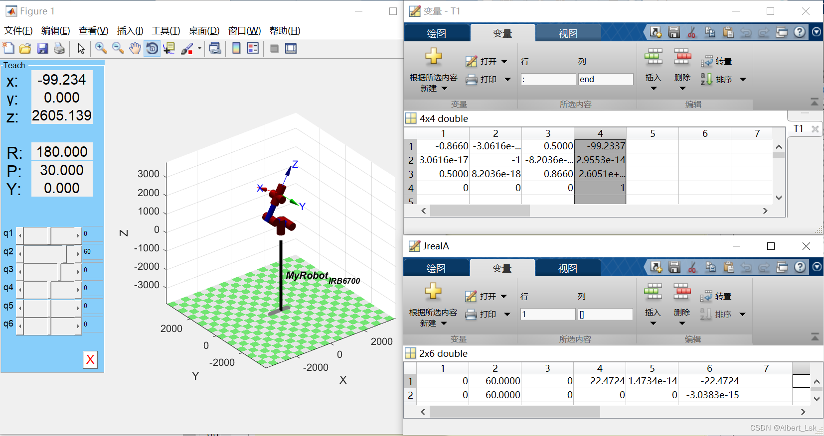
我们可以看到，左侧机器人示教器中，第二根轴的角度设为 $60^{\circ}$ ，其位置矩阵为 $[- 99.234, 0, 2605.139]$ 。右上方正解的最后一列完全对应，右下方逆解得到的数值与输入的角度数一致，因此可知逆解程序完全可行。

总结

以上就是逆向运动学的内容，本文详细介绍了如何理解运动学逆解，以及对运动学逆解的求解方法的罗列及原理说明。最后对运动学逆解实现代码的编程，使逆解能够有效得到目标位姿所对应的各轴转角。

参考文献

本文链接：https://blog.csdn.net/AlbertDS/article/details/123679114

原作者删帖不实内容删帖广告或垃圾文章投诉

智能推荐

874计算机科学基础综合,2018年四川大学874计算机科学专业基础综合之计算机操作系统考研仿真模拟五套题...-程序员宅基地

文章浏览阅读1.1k次。一、选择题1．串行接口是指( )。A. 接口与系统总线之间串行传送，接口与I/0设备之间串行传送B. 接口与系统总线之间串行传送，接口与1/0设备之间并行传送C. 接口与系统总线之间并行传送，接口与I/0设备之间串行传送D. 接口与系统总线之间并行传送，接口与I/0设备之间并行传送【答案】C2．最容易造成很多小碎片的可变分区分配算法是( )。A. 首次适应算法B. 最佳适应算法..._874 计算机科学专业基础综合题型

XShell连接失败：Could not connect to '192.168.191.128' (port 22): Connection failed._could not connect to '192.168.17.128' (port 22): c-程序员宅基地

文章浏览阅读9.7k次，点赞5次，收藏15次。连接xshell失败，报错如下图，怎么解决呢。1、通过ps -e|grep ssh命令判断是否安装ssh服务2、如果只有客户端安装了，服务器没有安装，则需要安装ssh服务器，命令：apt-get install openssh-server3、安装成功之后，启动ssh服务，命令：/etc/init.d/ssh start4、通过ps -e|grep ssh命令再次判断是否正确启动..._could not connect to '192.168.17.128' (port 22): connection failed.

杰理之KeyPage【篇】_杰理空白芯片烧入key文件-程序员宅基地

文章浏览阅读209次。00000000_杰理空白芯片烧入key文件

一文读懂ChatGPT，满足你对chatGPT的好奇心_引发对chatgpt兴趣的表述-程序员宅基地

文章浏览阅读475次。2023年初，“ChatGPT”一词在社交媒体上引起了热议，人们纷纷探讨它的本质和对社会的影响。就连央视新闻也对此进行了报道。作为新传专业的前沿人士，我们当然不能忽视这一热点。本文将全面解析ChatGPT，打开“技术黑箱”，探讨它对新闻与传播领域的影响。_引发对chatgpt兴趣的表述

中文字符频率统计python_用Python数据分析方法进行汉字声调频率统计分析-程序员宅基地

文章浏览阅读259次。用Python数据分析方法进行汉字声调频率统计分析木合塔尔·沙地克;布合力齐姑丽·瓦斯力【期刊名称】《电脑知识与技术》【年(卷),期】2017(013)035【摘要】该文首先用Python程序,自动获取基本汉字字符集中的所有汉字,然后用汉字拼音转换工具pypinyin把所有汉字转换成拼音,最后根据所有汉字的拼音声调,统计并可视化拼音声调的占比.【总页数】2页(13-14)【关键词】数据分析;数据可..._汉字声调频率统计

linux输出信息调试信息重定向-程序员宅基地

文章浏览阅读64次。最近在做一个android系统移植的项目，所使用的开发板com1是调试串口，就是说会有uboot和kernel的调试信息打印在com1上（ttySAC0）。因为后期要使用ttySAC0作为上层应用通信串口，所以要把所有的调试信息都给去掉。参考网上的几篇文章，自己做了如下修改，终于把调试信息重定向到ttySAC1上了，在这做下记录。参考文章有：http://blog.csdn.net/longt..._嵌入式rootfs 输出重定向到/dev/console

随便推点

uniapp 引入iconfont图标库彩色symbol教程_uniapp symbol图标-程序员宅基地

文章浏览阅读1.2k次，点赞4次，收藏12次。1，先去iconfont登录，然后选择图标加入购物车 2，点击又上角车车添加进入项目我的项目中就会出现选择的图标 3，点击下载至本地，然后解压文件夹，然后切换到uniapp打开终端运行注：要保证自己电脑有安装node(没有安装node可以去官网下载Node.js 中文网)npm i -g iconfont-tools（mac用户失败的话在前面加个sudo，password就是自己的开机密码吧）4,终端切换到上面解压的文件夹里面，运行iconfont-tools 这些可以默认也可以自己命名（我是自己命名的_uniapp symbol图标

C、C++ 对于char和char[]的理解_c++ char-程序员宅基地

文章浏览阅读1.2w次，点赞25次，收藏192次。char*和char[]都是指针，指向第一个字符所在的地址，但char*是常量的指针，char[]是指针的常量_c++ char*

Sublime Text2 使用教程-程序员宅基地

文章浏览阅读930次。代码编辑器或者文本编辑器，对于程序员来说，就像剑与战士一样，谁都想拥有一把可以随心驾驭且锋利无比的宝剑，而每一位程序员，同样会去追求最适合自己的强大、灵活的编辑器，相信你和我一样，都不会例外。我用过的编辑器不少，真不少～但却没有哪款让我特别心仪的，直到我遇到了 Sublime Text 2 ！如果说“神器”是我能给予一款软件最高的评价，那么我很乐意为它封上这么一个称号。它小巧绿色且速度非

对10个整数进行按照从小到大的顺序排序用选择法和冒泡排序_对十个数进行大小排序java-程序员宅基地

文章浏览阅读4.1k次。一、选择法这是每一个数出来跟后面所有的进行比较。2.冒泡排序法，是两个相邻的进行对比。_对十个数进行大小排序java

物联网开发笔记——使用网络调试助手连接阿里云物联网平台（基于MQTT协议）_网络调试助手连接阿里云连不上-程序员宅基地

文章浏览阅读2.9k次。物联网开发笔记——使用网络调试助手连接阿里云物联网平台（基于MQTT协议）其实作者本意是使用4G模块来实现与阿里云物联网平台的连接过程，但是由于自己用的4G模块自身的限制，使得阿里云连接总是无法建立，已经联系客服返厂检修了，于是我在此使用网络调试助手来演示如何与阿里云物联网平台建立连接。一.准备工作1.MQTT协议说明文档（3.1.1版本）2.网络调试助手（可使用域名与服务器建立连接）PS：与阿里云建立连解释，最好使用域名来完成连接过程，而不是使用IP号。这里我跟阿里云的售后工程师咨询过，表示对应_网络调试助手连接阿里云连不上

＜＜＜零基础C++速成＞＞＞_无c语言基础c++期末速成-程序员宅基地

文章浏览阅读544次，点赞5次，收藏6次。运算符与表达式任何高级程序设计语言中，表达式都是最基本的组成部分，可以说C++中的大部分语句都是由表达式构成的。_无c语言基础c++期末速成