【吴恩达深度学习】Deep Neural Network for Image Classification: Application-程序员宅基地
技术标签: 人工智能,机器学习,深度学习 算法 深度学习 人工智能
Deep Neural Network for Image Classification: Application
When you finish this, you will have finished the last programming assignment of Week 4, and also the last programming assignment of this course!
You will use the functions you’d implemented in the previous assignment to build a deep network, and apply it to cat vs non-cat classification. Hopefully, you will see an improvement in accuracy relative to your previous logistic regression implementation.
After this assignment you will be able to:
- Build and apply a deep neural network to supervised learning.
Let’s get started!
1 - Packages
Let’s first import all the packages that you will need during this assignment.
- numpy is the fundamental package for scientific computing with Python.
- matplotlib is a library to plot graphs in Python.
- h5py is a common package to interact with a dataset that is stored on an H5 file.
- PIL and scipy are used here to test your model with your own picture at the end.
- dnn_app_utils provides the functions implemented in the “Building your Deep Neural Network: Step by Step” assignment to this notebook.
- np.random.seed(1) is used to keep all the random function calls consistent. It will help us grade your work.
import time
import numpy as np
import h5py
import matplotlib.pyplot as plt
import scipy
from PIL import Image
from scipy import ndimage
from dnn_app_utils_v2 import *

%matplotlib inline
plt.rcParams['figure.figsize'] = (5.0, 4.0) # set default size of plots
plt.rcParams['image.interpolation'] = 'nearest'
plt.rcParams['image.cmap'] = 'gray'

%load_ext autoreload
%autoreload 2

np.random.seed(1)
2 - Dataset
You will use the same “Cat vs non-Cat” dataset as in “Logistic Regression as a Neural Network” (Assignment 2). The model you had built had 70% test accuracy on classifying cats vs non-cats images. Hopefully, your new model will perform a better!
Problem Statement: You are given a dataset (“data.h5”) containing:
- a training set of m_train images labelled as cat (1) or non-cat (0)
- a test set of m_test images labelled as cat and non-cat
- each image is of shape (num_px, num_px, 3) where 3 is for the 3 channels (RGB).
Let’s get more familiar with the dataset. Load the data by running the cell below.
train_x_orig, train_y, test_x_orig, test_y, classes = load_data()
The following code will show you an image in the dataset. Feel free to change the index and re-run the cell multiple times to see other images.
# Example of a picture
index = 7
plt.imshow(train_x_orig[index])
print ("y = " + str(train_y[0,index]) + ". It's a " + classes[train_y[0,index]].decode("utf-8") +  " picture.")
# Explore your dataset
m_train = train_x_orig.shape[0]
num_px = train_x_orig.shape[1]
m_test = test_x_orig.shape[0]

print ("Number of training examples: " + str(m_train))
print ("Number of testing examples: " + str(m_test))
print ("Each image is of size: (" + str(num_px) + ", " + str(num_px) + ", 3)")
print ("train_x_orig shape: " + str(train_x_orig.shape))
print ("train_y shape: " + str(train_y.shape))
print ("test_x_orig shape: " + str(test_x_orig.shape))
print ("test_y shape: " + str(test_y.shape))
As usual, you reshape and standardize the images before feeding them to the network. The code is given in the cell below.
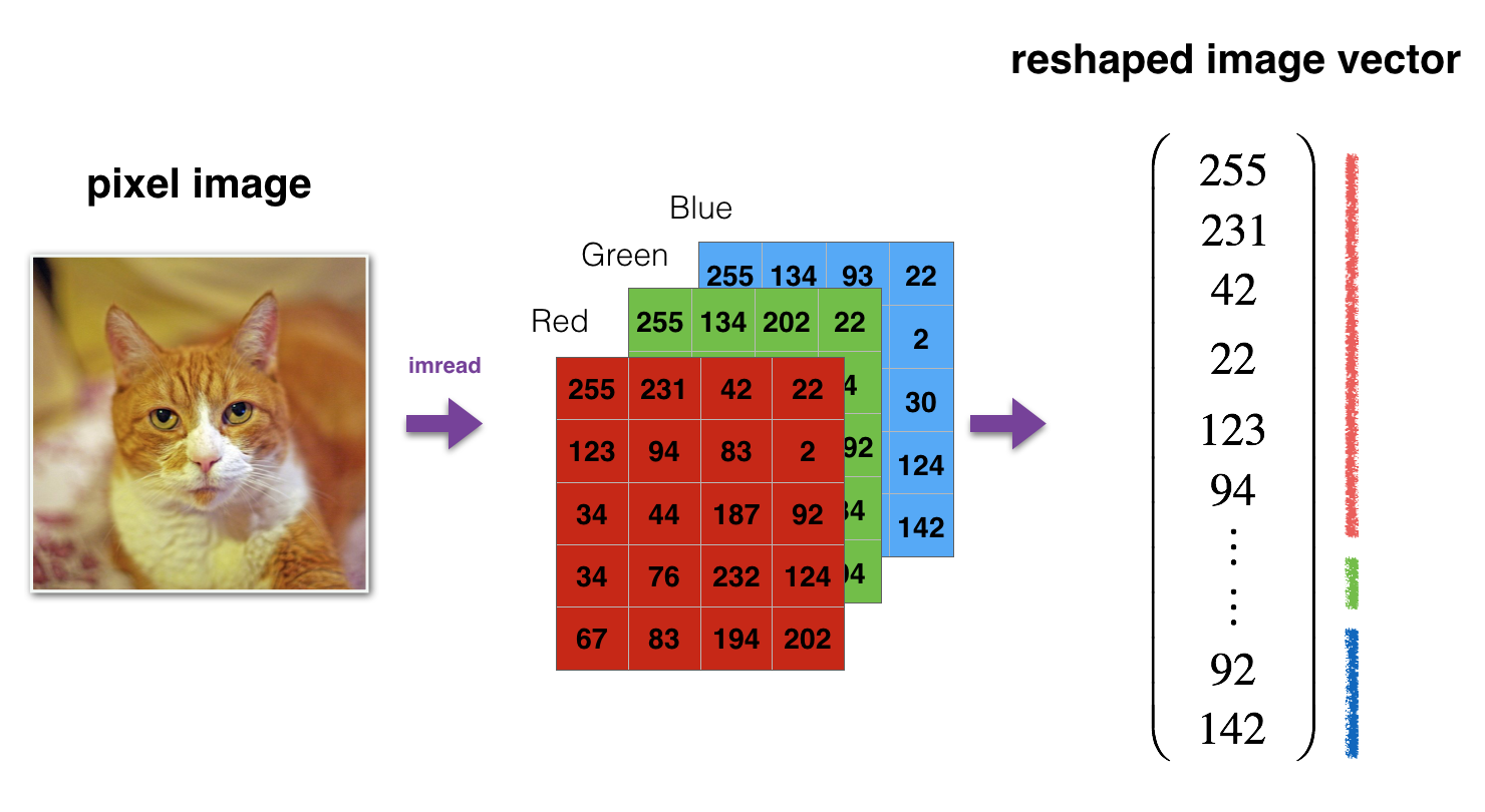
# Reshape the training and test examples
train_x_flatten = train_x_orig.reshape(train_x_orig.shape[0], -1).T   # The "-1" makes reshape flatten the remaining dimensions
test_x_flatten = test_x_orig.reshape(test_x_orig.shape[0], -1).T

# Standardize data to have feature values between 0 and 1.
train_x = train_x_flatten/255.
test_x = test_x_flatten/255.

print ("train_x's shape: " + str(train_x.shape))
print ("test_x's shape: " + str(test_x.shape))
12 , 288 12,288 12,288 equals 64 × 64 × 3 64 \times 64 \times 3 64×64×3 which is the size of one reshaped image vector.
3 - Architecture of your model
Now that you are familiar with the dataset, it is time to build a deep neural network to distinguish cat images from non-cat images.
You will build two different models:
- A 2-layer neural network
- An L-layer deep neural network
You will then compare the performance of these models, and also try out different values for L L L.
Let’s look at the two architectures.
3.1 - 2-layer neural network
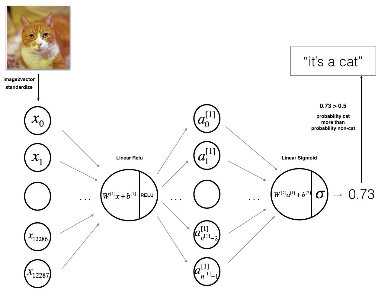
The model can be summarized as: ***INPUT -> LINEAR -> RELU -> LINEAR -> SIGMOID -> OUTPUT***.
Detailed Architecture of figure 2:
- The input is a (64,64,3) image which is flattened to a vector of size ( 12288 , 1 ) (12288,1) (12288,1).
- The corresponding vector: [ x 0 , x 1 , . . . , x 12287 ] T [x_0,x_1,...,x_{12287}]^T [x0,x1,...,x12287]T is then multiplied by the weight matrix W [ 1 ] W^{[1]} W[1] of size ( n [ 1 ] , 12288 ) (n^{[1]}, 12288) (n[1],12288).
- You then add a bias term and take its relu to get the following vector: [ a 0 [ 1 ] , a 1 [ 1 ] , . . . , a n [ 1 ] − 1 [ 1 ] ] T [a_0^{[1]}, a_1^{[1]},..., a_{n^{[1]}-1}^{[1]}]^T [a0[1],a1[1],...,an[1]−1[1]]T.
- You then repeat the same process.
- You multiply the resulting vector by W [ 2 ] W^{[2]} W[2] and add your intercept (bias).
- Finally, you take the sigmoid of the result. If it is greater than 0.5, you classify it to be a cat.
3.2 - L-layer deep neural network
It is hard to represent an L-layer deep neural network with the above representation. However, here is a simplified network representation:
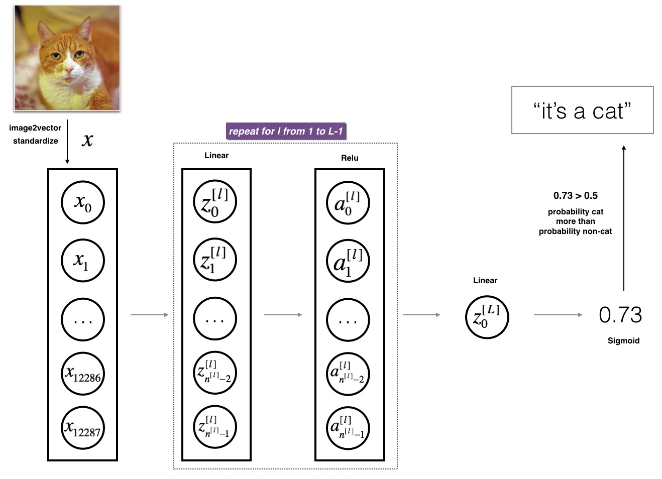
The model can be summarized as: ***[LINEAR -> RELU] $\times$ (L-1) -> LINEAR -> SIGMOID***
Detailed Architecture of figure 3:
- The input is a (64,64,3) image which is flattened to a vector of size (12288,1).
- The corresponding vector: [ x 0 , x 1 , . . . , x 12287 ] T [x_0,x_1,...,x_{12287}]^T [x0,x1,...,x12287]T is then multiplied by the weight matrix W [ 1 ] W^{[1]} W[1] and then you add the intercept b [ 1 ] b^{[1]} b[1]. The result is called the linear unit.
- Next, you take the relu of the linear unit. This process could be repeated several times for each ( W [ l ] , b [ l ] ) (W^{[l]}, b^{[l]}) (W[l],b[l]) depending on the model architecture.
- Finally, you take the sigmoid of the final linear unit. If it is greater than 0.5, you classify it to be a cat.
3.3 - General methodology
As usual you will follow the Deep Learning methodology to build the model:
1. Initialize parameters / Define hyperparameters
2. Loop for num_iterations:
a. Forward propagation
b. Compute cost function
c. Backward propagation
d. Update parameters (using parameters, and grads from backprop)
4. Use trained parameters to predict labels
Let’s now implement those two models!
4 - Two-layer neural network
Question: Use the helper functions you have implemented in the previous assignment to build a 2-layer neural network with the following structure: LINEAR -> RELU -> LINEAR -> SIGMOID. The functions you may need and their inputs are:
def initialize_parameters(n_x, n_h, n_y):
    ...
    return parameters
def linear_activation_forward(A_prev, W, b, activation):
    ...
    return A, cache
def compute_cost(AL, Y):
    ...
    return cost
def linear_activation_backward(dA, cache, activation):
    ...
    return dA_prev, dW, db
def update_parameters(parameters, grads, learning_rate):
    ...
    return parameters
### CONSTANTS DEFINING THE MODEL ####
n_x = 12288     # num_px * num_px * 3
n_h = 7
n_y = 1
layers_dims = (n_x, n_h, n_y)
# GRADED FUNCTION: two_layer_model

def two_layer_model(X, Y, layers_dims, learning_rate = 0.0075, num_iterations = 3000, print_cost=False):
    """
    Implements a two-layer neural network: LINEAR->RELU->LINEAR->SIGMOID.

    Arguments:
    X -- input data, of shape (n_x, number of examples)
    Y -- true "label" vector (containing 0 if cat, 1 if non-cat), of shape (1, number of examples)
    layers_dims -- dimensions of the layers (n_x, n_h, n_y)
    num_iterations -- number of iterations of the optimization loop
    learning_rate -- learning rate of the gradient descent update rule
    print_cost -- If set to True, this will print the cost every 100 iterations

    Returns:
    parameters -- a dictionary containing W1, W2, b1, and b2
    """

    np.random.seed(1)
    grads = {
    }
    costs = []                              # to keep track of the cost
    m = X.shape[1]                           # number of examples
    (n_x, n_h, n_y) = layers_dims

    # Initialize parameters dictionary, by calling one of the functions you'd previously implemented
    ### START CODE HERE ### (≈ 1 line of code)
    parameters=initialize_parameters(n_x,n_h,n_y)
    ### END CODE HERE ###

    # Get W1, b1, W2 and b2 from the dictionary parameters.
    W1 = parameters["W1"]
    b1 = parameters["b1"]
    W2 = parameters["W2"]
    b2 = parameters["b2"]

    # Loop (gradient descent)

    for i in range(0, num_iterations):

        # Forward propagation: LINEAR -> RELU -> LINEAR -> SIGMOID. Inputs: "X, W1, b1". Output: "A1, cache1, A2, cache2".
        ### START CODE HERE ### (≈ 2 lines of code)
        A1,cache1=linear_activation_forward(X,W1,b1,activation="relu")
        A2,cache2=linear_activation_forward(A1,W2,b2,activation="sigmoid")
        ### END CODE HERE ###

        # Compute cost
        ### START CODE HERE ### (≈ 1 line of code)
        cost=compute_cost(A2,Y)
        ### END CODE HERE ###

        # Initializing backward propagation
        dA2 = - (np.divide(Y, A2) - np.divide(1 - Y, 1 - A2))

        # Backward propagation. Inputs: "dA2, cache2, cache1". Outputs: "dA1, dW2, db2; also dA0 (not used), dW1, db1".
        ### START CODE HERE ### (≈ 2 lines of code)
        dA1,dW2,db2=linear_activation_backward(dA2,cache2,activation="sigmoid")
        dA0,dW1,db1=linear_activation_backward(dA1,cache1,activation="relu")
        ### END CODE HERE ###

        # Set grads['dWl'] to dW1, grads['db1'] to db1, grads['dW2'] to dW2, grads['db2'] to db2
        grads['dW1'] = dW1
        grads['db1'] = db1
        grads['dW2'] = dW2
        grads['db2'] = db2

        # Update parameters.
        ### START CODE HERE ### (approx. 1 line of code)
        parameters=update_parameters(parameters,grads,learning_rate)
        ### END CODE HERE ###

        # Retrieve W1, b1, W2, b2 from parameters
        W1 = parameters["W1"]
        b1 = parameters["b1"]
        W2 = parameters["W2"]
        b2 = parameters["b2"]

        # Print the cost every 100 training example
        if print_cost and i % 100 == 0:
            print("Cost after iteration {}: {}".format(i, np.squeeze(cost)))
        if print_cost and i % 100 == 0:
            costs.append(cost)

    # plot the cost

    plt.plot(np.squeeze(costs))
    plt.ylabel('cost')
    plt.xlabel('iterations (per tens)')
    plt.title("Learning rate =" + str(learning_rate))
    plt.show()

    return parameters
Run the cell below to train your parameters. See if your model runs. The cost should be decreasing. It may take up to 5 minutes to run 2500 iterations. Check if the “Cost after iteration 0” matches the expected output below, if not click on the square () on the upper bar of the notebook to stop the cell and try to find your error.
parameters = two_layer_model(train_x, train_y, layers_dims = (n_x, n_h, n_y), num_iterations = 2500, print_cost=True)
Expected Output:
| **Cost after iteration 0** | 0.6930497356599888 |
| **Cost after iteration 100** | 0.6464320953428849 |
| **...** | ... |
| **Cost after iteration 2400** | 0.048554785628770206 |
Good thing you built a vectorized implementation! Otherwise it might have taken 10 times longer to train this.
Now, you can use the trained parameters to classify images from the dataset. To see your predictions on the training and test sets, run the cell below.
predictions_train = predict(train_x, train_y, parameters)
Expected Output:
| **Accuracy** | 0.9999999999999998 |
predictions_test = predict(test_x, test_y, parameters)
Expected Output:
| **Accuracy** | 0.72 |
Note: You may notice that running the model on fewer iterations (say 1500) gives better accuracy on the test set. This is called “early stopping” and we will talk about it in the next course. Early stopping is a way to prevent overfitting.
Congratulations! It seems that your 2-layer neural network has better performance (72%) than the logistic regression implementation (70%, assignment week 2). Let’s see if you can do even better with an L L L-layer model.
5 - L-layer Neural Network
Question: Use the helper functions you have implemented previously to build an L L L-layer neural network with the following structure: [LINEAR -> RELU] × \times ×(L-1) -> LINEAR -> SIGMOID. The functions you may need and their inputs are:
def initialize_parameters_deep(layer_dims):
    ...
    return parameters
def L_model_forward(X, parameters):
    ...
    return AL, caches
def compute_cost(AL, Y):
    ...
    return cost
def L_model_backward(AL, Y, caches):
    ...
    return grads
def update_parameters(parameters, grads, learning_rate):
    ...
    return parameters
### CONSTANTS ###
layers_dims = [12288, 20, 7, 5, 1] #  5-layer model
# GRADED FUNCTION: L_layer_model

def L_layer_model(X, Y, layers_dims, learning_rate = 0.0075, num_iterations = 3000, print_cost=False):#lr was 0.009
    """
    Implements a L-layer neural network: [LINEAR->RELU]*(L-1)->LINEAR->SIGMOID.

    Arguments:
    X -- data, numpy array of shape (number of examples, num_px * num_px * 3)
    Y -- true "label" vector (containing 0 if cat, 1 if non-cat), of shape (1, number of examples)
    layers_dims -- list containing the input size and each layer size, of length (number of layers + 1).
    learning_rate -- learning rate of the gradient descent update rule
    num_iterations -- number of iterations of the optimization loop
    print_cost -- if True, it prints the cost every 100 steps

    Returns:
    parameters -- parameters learnt by the model. They can then be used to predict.
    """

    np.random.seed(1)
    costs = []                         # keep track of cost

    # Parameters initialization.
    ### START CODE HERE ###
    parameters=initialize_parameters_deep(layers_dims)
    ### END CODE HERE ###

    # Loop (gradient descent)
    for i in range(0, num_iterations):

        # Forward propagation: [LINEAR -> RELU]*(L-1) -> LINEAR -> SIGMOID.
        ### START CODE HERE ### (≈ 1 line of code)
        AL,caches=L_model_forward(X,parameters)
        ### END CODE HERE ###

        # Compute cost.
        ### START CODE HERE ### (≈ 1 line of code)
        cost=compute_cost(AL,Y)
        ### END CODE HERE ###

        # Backward propagation.
        ### START CODE HERE ### (≈ 1 line of code)
        grads=L_model_backward(AL,Y,caches)
        ### END CODE HERE ###

        # Update parameters.
        ### START CODE HERE ### (≈ 1 line of code)
        parameters=update_parameters(parameters,grads,learning_rate)
        ### END CODE HERE ###

        # Print the cost every 100 training example
        if print_cost and i % 100 == 0:
            print ("Cost after iteration %i: %f" %(i, cost))
        if print_cost and i % 100 == 0:
            costs.append(cost)

    # plot the cost
    plt.plot(np.squeeze(costs))
    plt.ylabel('cost')
    plt.xlabel('iterations (per tens)')
    plt.title("Learning rate =" + str(learning_rate))
    plt.show()

    return parameters
You will now train the model as a 5-layer neural network.
Run the cell below to train your model. The cost should decrease on every iteration. It may take up to 5 minutes to run 2500 iterations. Check if the “Cost after iteration 0” matches the expected output below, if not click on the square () on the upper bar of the notebook to stop the cell and try to find your error.
parameters = L_layer_model(train_x, train_y, layers_dims, num_iterations = 2500, print_cost = True)
Expected Output:
| **Cost after iteration 0** | 0.771749 |
| **Cost after iteration 100** | 0.672053 |
| **...** | ... |
| **Cost after iteration 2400** | 0.092878 |
pred_train = predict(train_x, train_y, parameters)
| **Train Accuracy** | 0.985645933014 |
pred_test = predict(test_x, test_y, parameters)
Expected Output:
| **Test Accuracy** | 0.8 |
This is good performance for this task. Nice job!
Though in the next course on “Improving deep neural networks” you will learn how to obtain even higher accuracy by systematically searching for better hyperparameters (learning_rate, layers_dims, num_iterations, and others you’ll also learn in the next course).
6) Results Analysis
First, let’s take a look at some images the L-layer model labeled incorrectly. This will show a few mislabeled images.
print_mislabeled_images(classes, test_x, test_y, pred_test)
A few type of images the model tends to do poorly on include:
- Cat body in an unusual position
- Cat appears against a background of a similar color
- Unusual cat color and species
- Camera Angle
- Brightness of the picture
- Scale variation (cat is very large or small in image)
7) Test with your own image (optional/ungraded exercise)
Congratulations on finishing this assignment. You can use your own image and see the output of your model. To do that:
1. Click on “File” in the upper bar of this notebook, then click “Open” to go on your Coursera Hub.
2. Add your image to this Jupyter Notebook’s directory, in the “images” folder
3. Change your image’s name in the following code
4. Run the code and check if the algorithm is right (1 = cat, 0 = non-cat)!
## START CODE HERE ##


## END CODE HERE ##

fname = "images/" + my_image
image = np.array(plt.imread(fname))
my_image = scipy.misc.imresize(image, size=(num_px,num_px)).reshape((num_px*num_px*3,1))
my_predicted_image = predict(my_image, my_label_y, parameters)

plt.imshow(image)
print ("y = " + str(np.squeeze(my_predicted_image)) + ", your L-layer model predicts a \"" + classes[int(np.squeeze(my_predicted_image)),].decode("utf-8") +  "\" picture.")
智能推荐
在类Unix平台实现TCP客户端-程序员宅基地
文章浏览阅读1k次,点赞8次,收藏16次。我们这个TCP客户端将从命令行接收两个参数,一个是IP地址或域名,另一个是端口,并尝试连接在这个IP地址的TCP服务端。
彩虹外链网盘界面UI美化版超级简洁好看-程序员宅基地
文章浏览阅读114次。彩虹外链网盘,是一款PHP网盘与外链分享程序,支持所有格式文件的上传,可以生成文件外链、图片外链、音乐视频外链,生成外链同时自动生成相应的UBB代码和HTML代码,还可支持文本、图片、音乐、视频在线预览,这不仅仅是一个网盘,更是一个图床亦或是音乐在线试听网站。适合小文件快速共享,文件可以设置访问密码,doc,图片等文件可以预览,音频可以在线播放,也适合做图床,支持在线下载,美化前台UI,运行天数和友链在后台统计代码修改。访问后台/admin 默认账号密码admin/123456。
vue项目启动不显示Network,及Network无法访问的问题_vue network网址访问不了-程序员宅基地
文章浏览阅读4k次,点赞2次,收藏15次。首先找到build文件夹下webpack.dev.conf.js文件,修改compilationSuccessInfo里边的messages属性。在vue.config.js(或者配置config了的,就在config下的index.js )文件下设置。最后在package.json文件中 scripts 下的 dev 或者 serve 后面加上。以上设置可以显示Network 调试地址,但是无法访问,还需设置一下。回车后会出现一串信息,复制IPV4 地址即可。地址 ,获取IPV4 地址方法,_vue network网址访问不了
C++cin.getline和std::getline的用法和区别-程序员宅基地
文章浏览阅读632次。从文件或控制台读入数据。都可以一次性读入多个字符,即读一串字符。cin.getline 是类函数。是基本输入流的函数。标准输入流,是一个类对象。也可以是。std::getline 是标准函数,使用时需要引入头文件 。cin.getline读入的数据一般放在字符数组中,std::getline读入的数据一般放在string对象中。由于cin.getline函数读入的数据放在字符数组中,所以要给出读入字符的(最大)数量。std::getline函数需要给出读入的文件流对象。 : 指向要存储字符到的字符数组的_std::getline
倍福--EL2521控制步进_倍福el2521接线图-程序员宅基地
文章浏览阅读944次。使用了EL2521控制步进电机。对于脉冲型步进或伺服驱动器,可使用EL2521模块控制操作流程1.1. EL2521简介1.1.1. 外观和接线EL2521 xxxx输出端子改变二进制信号的频率并输出(与K总线电气隔离)。频率由来自自动化设备的16位值预设。EtherCAT端子的信号状态由发光二极管指示。LED与输出同步,每个LED显示一个活动输出。1.1.2. EL2521信号类型EL2521模块的后缀有-0000,-0024,-0025,-0124几种,各种类型的接线是不同的,这点要稍_倍福el2521接线图
转载-mac下完全卸载Node.js(亲测可用)_mac 卸载 node.js-程序员宅基地
文章浏览阅读46次。【代码】转载-mac下完全卸载Node.js(亲测可用)_mac 卸载 node.js
随便推点
变色龙哈希函数 Chameleon Hash 可变型区块链_变色龙哈希改写区块-程序员宅基地
文章浏览阅读1.3w次,点赞7次,收藏42次。哈希函数 Hash:众所周知,区块链有着极其优秀的安全性就是因为其充分使用了哈希函数。哈希简单用一句话来讲,就是:将任意长度输入的字串可转换成一个固定长度的字串,通过原始字串可以很容易地算出转换后的字串,通过转换后的字串很难还原出原始字串。哈希函数特征:1. 对于任意m作为输入,得到输出的结果,很难找到另一个输入m' (m'不等于m),使得m'的Hash结果也为同样的输出_变色龙哈希改写区块
【LSTM回归预测】基于蜣螂算法优化长短时记忆DBO-LSTM风电数据预测(含前后对比)附Matlab代码-程序员宅基地
文章浏览阅读796次,点赞13次,收藏17次。基于蜣螂算法优化长短时记忆(DBO-LSTM)模型的风电数据预测是一个备受关注的研究领域。风电是一种清洁能源,其预测对于能源规划和市场运营具有重要意义。本文旨在通过对比蜣螂算法优化前后的长短时记忆(DBO-LSTM)模型在风电数据预测中的表现,探讨蜣螂算法在优化风电数据预测模型中的有效性。首先,长短时记忆(LSTM)是一种适用于时间序列数据的深度学习模型,它能够捕捉数据中的长期依赖关系,因此在风电数据预测中具有较好的表现。
小米便签data包源码解读_小米便签开源代码注释-程序员宅基地
文章浏览阅读1.8k次,点赞36次,收藏53次。对于小米便签data包源码的一些解读,可能不是很准确_小米便签开源代码注释
KE分析之slub_debug功能使用记录_photonicmodulat-程序员宅基地
文章浏览阅读2.1k次。1. 前记前段时间遇到一个问题,具有一定的代表性,特此记录,后续遇到类似问题时,可以参考这个方向2. 问题说明此问题为低概率煲机测试类问题,概率较低,需要长时间的运行才可以触发到,排查起来比较困难;2.1 测试方法设置机器为自动化休眠唤醒测试,时间周期为1分钟;usb 口有连接u盘,唤醒后会自动播放u盘内歌曲;无其他特别步骤测试时通过串口打印debug信息,另外打开系统中集成的debug功能,即收集logcat + kernel log信息,在遇到anr\je\ne\ke\hwt时会将现场_photonicmodulat
Spring + spring Mvc No Servlet Set 错误_no servletcontext set-程序员宅基地
文章浏览阅读60次。在使用注解开发,SpringMvc配置类的情况下开启@EnableWebMvc,如果在springConfig类中的@Component扫描Bean对象再次扫描到spring和springMvc的配置Bean对象就会出现No Servlet Set错误。_no servletcontext set
初学cesium时的一些笔记,过于潦草看看就好_cesium pbr 3200-程序员宅基地
文章浏览阅读840次。Cesium ion(假如要用自己的数据则需要上传数据)Cesium依赖:基于HTML5标准,无插件,跨平台;无法单独运行,依赖于浏览器(Cesium Lab基于Electron架构)浏览器基于HTTP协议,所以必须有HTTP ServerCesium功能介绍:定义影像矢量模型:{1使用3d tiles格式模式加载各种不同的3d数据,包含倾斜摄影模型,三位建筑物,CAD和BIM的外..._cesium pbr 3200